Skip navigation

So a few days ago I showed off some results of using a line profiler package to get detailed feedback on python programs.  Using the package, I found out that my cost calculation algorithm for a Tabu Search implementation for the Traveling Salesman Problem (TSP) was the major bottleneck in my code.  After playing around with the function and reading some forums, I figured out a way to significantly improve the cost function.  I was originally computing the cost of the entire TSP path for every 2-Opt iteration.  It turns out that this was a fairly excessive calculation, as I was only swapping the positions of two nodes at a time, the resulting change to the total cost was simply the distances between the two nodes and their respective neighbors.  So I modified the function to accept the position of the two nodes, and then calculated the distance of those partial routes to identify swaps that increased the solution’s optimality.

The original code is posted below.  In this function, I pass in a list of index values that correspond to the order in which the nodes are visited and then the function computes the total distance of the path, including the return trip to the starting point.

def calc_cost(perm):
	distance = length(points[perm[-1]], points[perm[0]])
	for i in range(0, nodeCount-1):
	    distance += length(points[perm[i]], points[perm[i+1]])
	return distance

In the modified function, shown below, I pass in the same list as before, however I added another argument to the function that indicates the position of the path that I want to evaluate. The function then calculates the distance between the provided position and the node directly before and after it in the path. I call this function four times when evaluating a 2-Opt iteration, twice to evaluate the change in the two points that were swapped, and twice again to evaluate the original distance in the path.  If the total segmented distance of the two swapped points is lower than the total segmented distance of the original two points, I keep the modified solution as it will have a lower total distance.

def calc_seg_cost(perm, c):
        if c != len(perm) - 1:
            seg = [perm[c-1], perm, perm]
        else:
            seg = [perm[c-1], perm, perm[0]]
        distance = 0
        for i in range(0, len(seg)-1):
            distance += length(points[seg[i]], points[seg[i+1]])
        return distance

I ran the two different versions of the code on a number of TSP problems and recorded the time of each run using the unix time utility.  I then plotted the results using matplotlib.

time_plot

As you can see from the plot, the function modification appears to be saving a substantial amount of time.  The primary advantage of this modification is that I can run my algorithm for a higher number of iterations and get better optimatily in the 5 hour time frame that we have.  This should help me improve my scores, but I may still need to keep tweaking the algorithm if I want to get higher scores on the larger problems, as it looks like the cost function modification by itself will not be enough to achieve that goal.

So as I mentioned in my last post, I am currently taking a discrete optimization class from Coursera.  It is a pretty challenging class, especially because I have never taken an algorithms class before (I majored in Conservation and Resource Studies in college).  I have been fairly successful in implementing some tried and true algorithms to solve some of the problem sets, but I have been having a lot of difficulty getting an understanding of the performance details of the various algorithms.  My typical routine has been to write up a few solutions to each problem, and use the run-time, solution score, and my (limited) intuition to try and improve the implementations.

In yesterday’s post I discussed a little plotting function that I wrote to help visualize my implementations to the Traveling Salesman Problem (TSP).  Today, I am going to talk about using a line profiler to get detailed feedback on the performance of your code.  I found this blog post to be very helpful in navigating the various options for performance analysis.

For the (TSP) problem, I wrote up a Tabu Search algorithm, which is a type of Local Search algorithm, that uses ‘short term memory’ to ensure that old solutions are not revisited.  While I have successfully implemented a version of the algorithm in python, I am fairly certain that I am glossing over a few key implementation details as my algorithm is not performing nearly as well as it should.  A good way to get detailed feedback on the algorithm’s performance is to use the line profiler package.  It is extremely easy to use and it provides valuable feedback on your code’s performance.  You simply add the @profile decorator to any function in your program that you want feedback on, then run a python executable at the command line (see the source blog post for details).  I threw in the profile decorator on my main Tabu function and got the following output:

Line #      Hits         Time  Per Hit   % Time  Line Contents
==============================================================
    85                                               @profile
    86                                               def search(cities, candidate_list_size, max_iter):
    87         1        13160  13160.0      0.1  	current_vector = random_permutation()
    88         1          839    839.0      0.0  	current_cost = calc_cost(current_vector)
    89         1            3      3.0      0.0  	tabu_list = []
    90         1            5      5.0      0.0  	path = [current_vector[:]]
    91     10001        30512      3.1      0.3  	for i in range(0, max_iter):
    92     10000      9332657    933.3     99.1  	    new_perm, new_cost, tabu_list = generate_candidates(current_vector, tabu_list)
    93     10000        37371      3.7      0.4  	    if new_cost < current_cost:
    94                                           		#path.append(new_perm[:])
    95        11           53      4.8      0.0  		current_vector = new_perm[:]
    96        11           34      3.1      0.0  		current_cost = new_cost
    97         1            4      4.0      0.0  	return current_vector, current_cost, path

The output of the profiler displays Hits (which is the number of times a line of code was run), Time Per Hit, and % Time. Looking at the output from the profiler, it looks like the line of code that uses the most resources is the generate_candidates function call in the main for loop (which makes sense, as the search function is basically a for loop over the generate_candidates function . So in order to take this analysis further, I added a profile decorator to the generate_candidates function and displayed the results below.

Line #      Hits         Time  Per Hit   % Time  Line Contents
==============================================================
    74                                               @profile
    75                                               def generate_candidates(best_perm, tabu_list):
    76     10000        37295      3.7      0.4  	perm = best_perm[:]
    77     10326        29927      2.9      0.3  	while True:
    78     10326       426132     41.3      4.7  	    perm = two_opt(best_perm)
    79     10326        73413      7.1      0.8  	    if perm not in tabu_list:
    80     10000        95461      9.5      1.1  		tabu_list = tabu(perm, tabu_list)
    81     10000        28268      2.8      0.3  		break
    82     10000      8269102    826.9     92.0  	perm_cost = calc_cost(perm)
    83     10000        29902      3.0      0.3  	return perm, perm_cost, tabu_list

As you can see from the output of the profiler on the generate_candidates function, the bottleneck appears to be the calc_cost function. This was not surprising as cost functions, which are used to measure the effectiveness of your solution, can be expensive to compute but are an important tool in providing your algorithm feedback in order to direct it to an optimal solution.  In this case, the cost function is a simple for loop that calculates the distance traveled in a given solution, so if I want to improve upon it, I am going to need to figure out a better way to estimate or approximate the cost without having to do the full calculation.

So know that I know where my bottleneck is, I am going to get to work on trying to find a way to improve the algorithm so that I can get some good solutions for the problem sets.  I will post an update, with some comparative metrics on performance if/when I find a way to reduce the bottleneck.

So I am taking a discrete optimization class through Coursera and so far it has been pretty intense. The class uses python for it’s homework submission, so while you are free to use any language to solve the homeworks, it was easy to get up and running because python was well supported.  As I quickly found out however, the python language has a lot of overhead that slows it down considerably compared to other languages.  So I have been playing with Cython (a python package that tries to optimally compile python code to C) and have had some success with that, but will probably have to keep exploring other options as my code has been running horribly slow.

One of the recommendations from the professor was to use visualizations to help debug and improve algorithms.  I had been looking for an excuse to dive into the python plotting library matplotlib, and this seemed like a good excuse to do so. I was having trouble getting a feel for the performance of a Tabu Search implementation that I was working on for the Traveling Salesman Problems (TSP), so I decided to code something up using matplotlib to help me get a better idea of how the algorithm was working.

The TSP is a very difficult problem to optimize.  When the number of nodes gets very large, the amount of time it takes to find an optimal solution increases exponentially.  As such, it is often better to attempt to achieve sub-optimal solutions using Local Search techniques.  The downside to these algorithms, is that they rely on randomly searching for small improvements in the solution, and due to the randomness involved, it is difficult to get an idea of how your algorithm is working.  So this problem makes a fairly good candidate for developing supporting visualizations.

I took a stab at writing a simple plotting function that would plot out the nodes of the TSP problem as well as the solution path.  But I also wanted to compare the current solution with previous iterations to see how the algorithm was performing.  So I created a function that allows you to pass in as many iterations of the solutions as you like, and plots out the current solution, and overlays that on top of the older solutions in a different color.  I have used plotting libraries in R and SAS before so I figured this wouldn’t be too difficult, but as I quickly found out, and as anyone who has ever used a plotting library knows, it is pretty easy to get bogged down in documentation as each function/object has dozens of optional arguments (which is pretty standard for plotting libraries, as they need to provide the flexibility for users to create unique visualizations) and plenty of quirks.  One of the more frustrating issues that I ran into was I wanted to have arrows indicating the direction of travel to the individual nodes.  I spent a while trying to look if there was an optional line type I could use, but as I soon found out, I needed to call a special arrow object and individually draw each arrow between each point.  I was able to accomplish this with a couple of for loops, so it wasn’t a huge deal, but it definitely added to the verbosity of the code.  Anyway, the code is up on gist, here, and I have attached a few examples of the resulting output below.

There are a few things that I want to try and improve on when I get the time.  I could not find a way to lower the transparency of the arrows to represent older iterations of the solutions.  Instead, I decided to reduce the width of the red lines, however, it doesn’t seem to have a noticeable effect.  Also I wanted older iterations of the solution to have a red dashed line, but some of them appear to be solid lines.  From what I can tell, this looks like it is just an issue with the rendering.

So that’s it for today.  My next task is to play around with a line profiler to get a detailed breakdown about the performance of each line in my code.  Hopefully this will help me increase the performance of my algorithms enough to start actually getting some passing grades on the homeworks!


So I am apparently not very good at updating this blog.  I think part of the problem is I have been keeping pretty busy with Coursera classes, programming, and surfing.  When I initially started this blog, I envisioned that it would be a good way to document all of the little side projects I was working on, but I have been pretty bad about seeing these projects through to completion, so there hasn’t been much to show for the work so far.  So I am going to change directions a little bit, and probably start throwing snippets of code onto gist and write about it here.  Hopefully that will encourage me to write a few more posts!

One ‘project’ that I did manage to complete was to build a semi-functional desk from an old Ikea bed frame.  My roommate had upgraded his bed a few months ago and had initially planned on giving away or selling the old frame.  However, it just ended up sitting in a dis-assembled pile on our back porch, and I figured it would be a good idea to build something from it.  We have this weird nook in our living room that is curved, and it is difficult to efficiently use the space because most furniture items aren’t designed for that.  Additionally, due to the windows and the orientation, the space gets great natural light, so I figured it would make a good work space (I had originally setup the dining table there and was using that as a makeshift desk).

So after some back of the napkin plans my roommate and I got to work measuring, cutting, and assembling.  Out method was pretty ad hoc, and we weren’t quite sure our ‘design’ was going to actually be stable or strong enough, but after a few hours of grinding away, we ended up with something that resembled a desk!  We used the wooden slats from the bed frame to create the work surface, and offset them so that they would fit against the curve of the wall, which allowed the desk to fit snugly against the wall optimizing the space.  We cut up some of the support pieces of the bed frame for the legs.  Pictures of the before and after are below (note: the picture of the bed frame was pulled off the internet).

So after a month or two of use, I can safely say that the desk is sturdy enough (for the most part) to handle everyday use.  Some of the slats have come loose, so I need to be careful when leaning on the edge of the desk (as they might pop off).  The reason for this problem was we did not want to have screw heads exposed on the work surface, so we picked up some small screws from the hardware store and drilled through the bottom of the frame into the  bottom of the slats.  Unfortunately, our screws were a little to short, so each slat is only held on to the frame by a few screw threads, making it fairly easy to knock them loose.  I might go back with some wood glue at some point to add some extra fastening strength if the problem gets worse.

It was fun to break out the saw and the drill.  I used to build skate ramps as a young lad, and have always enjoyed woodworking, but you don’t get many opportunities for it when you live in a small-ish apartment in the middle of San Francisco.  Anyways, thanks to my roommate Will for working with this on me, hopefully I can use this desk to actually get some work done!

So in my last post, I wrote about the setup of my little CryptoCoin mining experiment, and in this post I am presenting the results.  But before I jump into the results, I want to discuss some of the assumptions and biases of this experiment:

Bitcoin and Litecoin both adjust the difficulty of their proof-of-work problems in order to throttle the mining process and keep the additions to the block chain occurring at a regular, predetermined rate.  The difficulty changes frequently, and over the course of the experiment, the difficulty for both Bitcoin and Litecoin increased significantly.  This means that the rate of coin mining most likely got a good deal slower as the experiment progressed. Unfortunately I did not collect interval data, I only have overall results, so I cannot quantify the impact (would make an interesting follow on, perhaps I will do it later).  If you attempt to recreate this test, your results will vary significantly due to this issue.

In addition to the variable difficulty, each mining pool has it’s own issues.  Both mining pools would go down from time to time (this is pretty common).  Unfortunately, when the Bitcoin pool would go down, the miner on the RasPi would shutdown. I did my best to check regularly and restart the miner (apparently there are ways to have the miner automatically switch to a backup pool), but there were definitely a few times when it went down for more than a day.  The impact is probably in the range of 10-20%, meaning had I taken better measures to protect against downtime, I most likely would have seen an increase in Bitcoin returns by 10-20%.

The final consideration to make, is that the value of the respective coins is constantly changing.  I used $127.53 for Bitcoin and $2.86 for Litecoin.  These were the prices of the coins on the day I stopped the experiment.  The exchange rates vary wildly, and as such, your results will depend heavily on the current exchange rates.

So let’s get down to it.  The experiment lasted 42.1 days (I let the miners run for a bit longer than I initially had planned).  The following table presents the number of coins mined and the dollar value of those coins:

results1

So as was expected, the RasPis mined much more Litecoin than Bitcoin over the course of the 42 days.  This is due to the popularity, and subsequently difficulty, of mining Bitcoin.  Interestingly enough, while we mined 2x orders of magnitude of Litecoin, due to the exchange rates of the coins, the monetary value of the coins was much closer.

Another factor that needs to be taken into account is the cost of electricity.  While, I am currently using the RasPis as servers and development/test boxes, if I wanted to use the RasPi as a dedicated mining rig, than I would need to adjust the returns for the cost of electricity required to run the device (while RasPis are really low powered, if you were running a dedicated GPU rig, electricity costs would be a very important factor to consider).  After digging around on the internet I came up with a rough estimate of the energy consumption of a RasPi.  Interestingly enough, the RasPi seems to have fairly stable power consumption regardless of the amount of processing it is doing (a testament to the efficiency of the ARM processors?).  I rounded the power consumption up to 3 watts (from 2.5) to keep things conservative.  Below is a breakdown of the costs, the electricity rate was pulled from my latest utility bill:

results2

And here is the electricity adjusted returns of the mining operation:

results3

 So as you can see, accounting for electricity costs, the miner operations for both Bitcoin and Litecoin resulted in negative returns.  As I mentioned, I have the RasPis up and running for other reasons anyway, but regardless, the number of coins mined are so small that the gains are entirely swamped out by electricity costs.  Just to break even, you would need Bitcoin to increase in value to ~$1950 and Litecoin to increase in value to ~$17.35.  And of course, that is assuming the mining difficulty stays relatively constant, which it most assuredly won’t if the exchange rate rises to those levels.

So in conclusion, if you were hoping to set up a Raspberry Pi CryptoCoin mining rig in order to retire early, I would recommend reconsidering, or at least keep your day job!  But if you have some Raspberry Pis up and running anyway, and want to play around with some of the mining software that is out there, than this is a good way to get into the game with out risking the security of your main computer (there are some pretty sketchy operators in the CryptoCoin space, so take precautions).

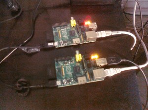
So while in Costa Rica for a surf trip, I thought it would be a fun project to run a little cryptocurrency mining experiment.  I have been playing around with a few Raspberry Pis for a while now, and out of curiosity decided to set them up as cryptocurrency miners.  Anyone who has been following the Bitcoin (BTC) craze as of late, and has a rough idea of how the mining process works, would know that using a Raspberry Pi as a Bitcoin miner is like bringing a knife to a gun fight (actually it is more like bringing a toothpick to a gun fight).  But considering I was going to be out of the country for two weeks with limited internet, I figured I might as well put the Raspberry Pis to some use.  After doing a little research, I decided to simultaneously run two Raspberry Pis as cryptocurrency miners, one mining Bitcoin, the other Litecoin, and after a few weeks of run time, evaluate and compare the rate of return on the two mining operations.

For this post, I am going to provide a quick background on the two coins and what this experiment will demonstrate.  I will write a separate follow up post with the results later.  There has been plenty of press on Bitcoin in the last month, so I won’t go into too much detail about what Bitcoin is, but for those who are not aware, there are also a number of alternative currencies in existence.  One of those currencies is called Litecoin (LTC).  The advocates of Litecoin advertise the project as ‘the silver to Bitcoin’s gold’.  Litecoin is one of a handful of alternative coins that has gained enough traction to get off the ground and it appears to be the most adopted of the alternative currencies.  The code for Litecoin was based on the Bitcoin protocol, but modified in a few ways to compensate for some of Bitcoin’s perceived shortcomings.

The primary difference between Bitcoin and Litecoin is the hashing algorithm used in the ‘proof of work‘ phase.  Bitcoin and Litecoin mining are done by solving complex problems called proof of work.  These proof of work problems are designed to require a fair amount of computing power to solve, however they are easily verifiable, so once a solution is found, it is easy for the network to verify that the solution is valid.  This is done by requiring miners to randomly seed a hashing algorithm until they get a certain output.  Once the appropriate seed value is found, the solution can be verified by others by simply using the solution seed and running it through the hashing algorithm to check that you get the appropriate output.

For those that aren’t familiar with hashing algorithms, a good analogy to this process is brute-force password cracking (i.e. randomly trying to guess someone’s password).  In order to guess someone’s password, you would have to try thousands upon thousands of iterations, but once the correct password is found, it is very easy for someone else to verify that you have found it.  The time it takes to find the correct password is fairly random, i.e. it is possible that you could guess it correctly on the first attempt, or it could take you millions of attempts.  Adding computing power to the problem will speed up the number of attempts you can make, but it does not guarantee that any individual attempt is more likely to succeed.

With Bitcoin and Litecoin mining, individual miners compete against each other to find the solution to the proof of work problem.  The first node that correctly finds the solution is rewarded with a number of coins.  Adding computational power to you miners increases the odds that you will find the solution first, but because of the randomness involved in the process, it does not guarantee that you will be the first to solve a particular proof of work.  As of late, Bicoin has faced something of an arms race.  Bitcoin uses the SHA256 hashing function in its proof of work.  This algorithm is highly parallelizable, which roughly means that throwing more computational power at the algorithm will result in faster iterations.  Graphical Processing Units (GPU’s) are very well suited to the task, and as such they quickly displaced CPU’s as the preferred Bitcoin mining hardware.  More recently, Field Programmable Gate Arrays (FPGAs) and Application Specific Integrated Circuits (ASICs) have taken over the mining scene.  FPGAs are programmable chips and ASICs are specially manufactured chips.  FPGA’s started coming online a year or so ago and displaced GPU’s.  ASICs are starting to appear in mining rigs and will eventually displace FPGA’s.  This arms race has largely left the average person standing on the sidelines, as profitable mining rigs now require fairly significant investments to obtain, and your average desktop computer, even if you use the GPU, is fairly useless as a miner, and in fact would probably result in a negative return on your investment after factoring in energy costs.

Litecoin was created in response to this arms race.  The designers of Litecoin were upset that Bitcoin mining had left the average user in the dust and felt that a cryptocurrency that was designed with a more level playing field would encourage wider adoption.  As such the designers of Litecoin forked the Bitcoin source code and modified the hashing algorithm used in the proof of work.  Instead of using the SHA256 function, they changed the code to use the scrypt hash function.  The reason, in short, for this change was that the scrypt algorithm is more memory intensive, and as such it is not as parallelizable as SHA256.  Therefore, simply adding more raw computational power, in theory, would not have as large of an impact as it would with the SHA256 algorithm.  This means that the gap between the hashing power of CPU’s, GPU’s, FPGA’s and ASIC’s is much narrower, thus giving the average person a better chance at staying in the game.

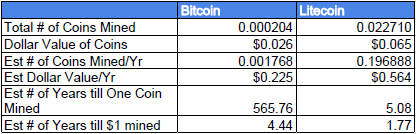
Considering this, I thought it would be fun to see how my Raspberry Pis would fare as miners for these two different currencies.  In theory, I should be able to mine much more Litecoin than Bitcoin, as the playing field is a little more level, and due to the lower popularity, there are fewer miners resulting in a lower overall network hash rate (its still like bringing a toothpick to a gunfight, but the guns are limited to single shot rifles, rather than semi-automatics, and there are fewer attendees overall!).  Of course, an additional factor that needs to be considered is the market price for each of the coins, as Bitcoin has been trading at over $100 whereas Litecoin has been trading for less than $5.  So while I will most likely mine more Litecoin than Bictoin, it is not yet clear which mining operation will result in the most ‘profit’.

In order to facilitate this experiment, it was necessary to sign up for mining pools for each of the currencies.  Mining pools are a way to aggregate computing resources in order to cooperatively mine the coins.  The major reason for doing this is because for most individuals, it is nearly impossible to successfully complete a proof of work (once again, the mining process is essentially a competition, where the first node to present a valid solution wins).  By joining a mining pool, you ensure that you will receive some form of payout, as the combined resources of the pool should be enough to successfully complete some proof of work, and when it does, the rewards are divided among the pool participants based upon the amount of hashing power they contributed.  For Bitcoin, I chose to use deepbit.net, and for Litecoin I chose to use notroll.in.  I am not endorsing either of these pools as I have not had much experience with either of them (anyone that is seriously considering mining coins should do some research into the pool they use, as there has been numerous reports of shady operators).

So the miners have been running for almost three weeks at this point.  I am going to tally up the numbers and post some results and analysis shortly.

Well, been plugging away a at a variety of projects, but for the most part I don’t have much to show… yet!  I ran through an in-depth Flask turorial (a light weight web framework for python) and am starting to put together a front end for one of the web scrappers I built.  Hopefully I will have that online soon.

In other news, this blog is no longer hosted on the Raspberry Pi.  I moved it over to a hosted solution.  Getting the pi up and running as a web server was a fun little introduction to the device, but ultimately I have a number of other projects I want to try out, and it made more sense to free up the Pi for those projects.  I have ordered two more Pis (for a grand total of four) and hope to play around with mesh networking and parallel computing, however in the mean time, I have set up the two Pis as Litecoin miners (more on that later).

In a few hours, I will be heading out to Costa Rica for a short surf trip, but will write up the Litecoin post while I am on the plane.

So I sort of got the DNS issues figured out.  Still working out a few kinks, and playing with wordpress themes as well.

I setup another Raspberry Pi server here.  Currently it is running a python/flask microblog site called Flaskr that is used as one of the example projects for learning flask.  Code pulled from here.  I will be playing around with some python/flask code over the next few days to setup a project site, so these links may not be working from time to time.  I will post an update once it is ready.

Well, sort of.  Still playing around with the DNS settings at my domain name host as the url isn’t redirecting properly. It took a few attempts to get this up and running, largely due to my unfamiliarity with LAMP.  Some tutorials were better than others, but this was the one that I ended up using.

20130310 RaspberryPi Setup