Skip navigation

Category Archives: gist

So one of my goals for the new year is to better document and present my side projects.  I have a habit of playing around with an idea and getting a very bare bones prototype, and then letting it sit and languish.  So to kick things off, I present to you Surf Check.

One of the first python programs I ever wrote was a surf scraping program that pulled surf forecast data from SwellIinfo.com, a surf forecast website, for 6 different locations and printed out a condensed surf report for all of the locations on a single page.  Besides getting experience with python, the main reason I wrote the code was because it was a pain to try and flip through a handful of surf forecast pages on the surf website.  The website is loaded with graphics and ads, and it is not easily navigable.  So a quick check of the surf forecast would end up taking over 5 minutes, accounting for page loads and navigation.  I figured building a scraper to grab the data I wanted and condense it down to one page was a perfect first project.

I wrote the initial scraper around March, 2013 when I was just getting started with Python. Overtime I tinkered around with the program, and eventually decided to re-write it and turn it into a small web page to make it easier to access.  So I added a flask server, re-wrote the scraper code, and set up a simple frontend with a jinga template serving basic html.

surfappscreenshot

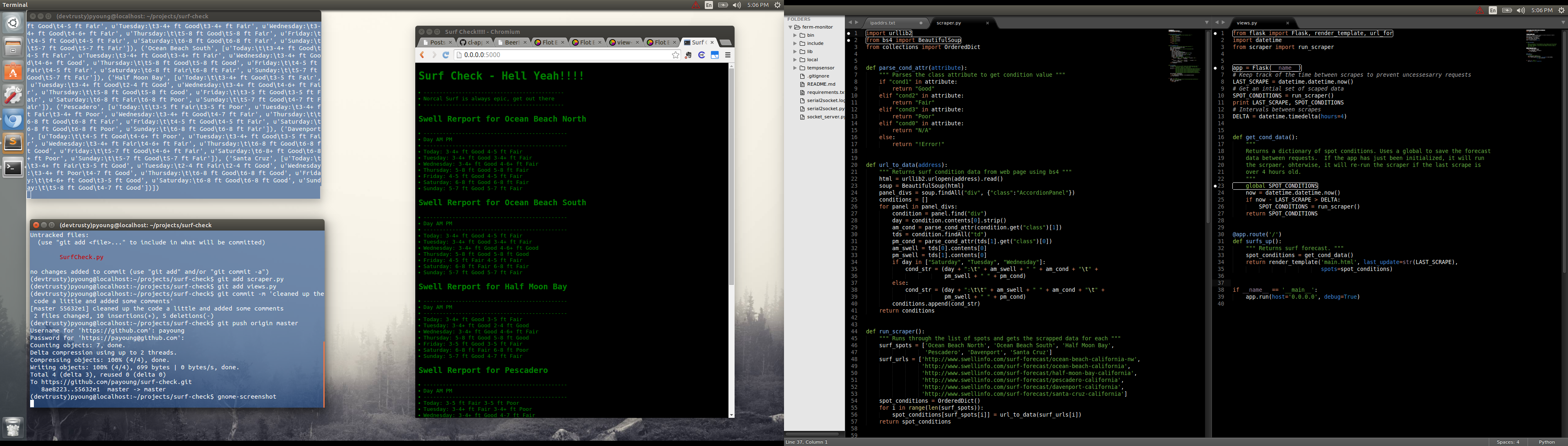
Screenshot of Surf Check Development

Comparing the before and after, I was able to make some pretty big improvements to the original code.  The original scraper was over 160 lines, and the new project is ~140 lines, including flask server, html template, and scraper.  Of course the comparison is thrown off by the fact that for some reason when I wrote the original program, I couldn’t get Beautiful Soup (a.k.a. bs4, a python html parser) to work.  My guess is it was due to my unfamiliarity with object oriented programming and python in general, but I did a weird workaround where I saved the bs4 output to a text file, imported the text file and then parsed the text to get what I needed.  Ahhh, yes, the things we do when we are inexperienced!  Makes me cringe now, but it is a good lesson.  Had I gotten bs4 to work the first time around, I am pretty sure the scraper code would have been pretty similar to my final version.

A quick note on the code for the project.  Below is the bulk of the code that makes up the views.py file.

app = Flask(__name__)
# Keep track of the time between scrapes to prevent uncessesarry requests
LAST_SCRAPE = datetime.datetime.now()
# Get an intial set of scaped data
SPOT_CONDITIONS = run_scraper()
print LAST_SCRAPE, SPOT_CONDITIONS
# Intervals between scrapes
DELTA = datetime.timedelta(hours=4)

def get_cond_data():
    """
    Returns a dictionary of spot conditions. Uses a global to save the forecast
    data between requests.  If the app has just been initialized, it will run
    the scrpaer, ohterwise, it will re-run the scraper if the last scrape is
    over 4 hours old.
    """
    global SPOT_CONDITIONS, LAST_SCRAPE
    now = datetime.datetime.now()
    if now - LAST_SCRAPE > DELTA:
        SPOT_CONDITIONS = run_scraper()
        LAST_SCRAPE = now
    return SPOT_CONDITIONS

@app.route('/')
def surfs_up():
    """ Returns surf forecast. """
    spot_conditions = get_cond_data()
    return render_template('main.html', last_update=str(LAST_SCRAPE),
                           spots=spot_conditions)

Scraping the forecast data from the surf website takes a while, ~9 seconds for all six pages.  If I was expecting a lot of traffic, I would set up a scheduler that would automatically scrape the site in the background so that the data would be available immediately when a request hit the server.  However, as this is just a small project that I am doing for fun, I don’t want to hit Swellinfo’s servers with excessive scrape requests.  So I decided to scrape only when a request was made to my site.  The obvious downside is that this results in a really long load time for the page, as it has to wait for the scrape to finish before it can serve the data.  To mitigate this issue slightly, and to further limit requests to Swellinfo’s servers, I store the forecast data for a period of time (surf forecasts typically only get updated every 12 hours or so).  At the moment, I have that period set to 4 hours, so if the scraped data is over four hours when a request hits my homepage, it will re-scrape the data, however every homepage request in the next 4 hours will get served the saved scraped data.  Additionally, to keep things simple I choose to forgo any persistent data storage.  So at the moment, the scraped data gets stored in a global variable (SPOT_CONDITIONS).  While using global variables in python are looked down, I thought it was an interesting way to change up the typical flasks MVC (Model-View-Controller) model.  Essentially I have just reduced it down to VC.

I thought that code snippet was fun because, despite it’s apparent simplicity, it hides some complex design decisions.  In the future, it might make sense to implement a more robust scraping mechanism, perhaps by figuring out the exact times that the Swellinfo surf forecasts get updated, and then only re-scraping if the data is old (instead of arbitrarily using the 4 hour cutoff).  I have a few ideas for improvements or features I would like to add to the site, but I also have some more ambitious projects on my plate that are hogging my attention, so well see if I get around to it.  If you want to check out either the old scraper code (my first python program) of this current iteration of the project, the links are here:  My First Python Program!!!  Surf Check Github Repo!!!!

In my continuing quest to improve my scores for the discrete optimization class, I stumbled upon a data structure called ‘k-d tree’ (short for k-dimensional tree).  Supposedly it is a really good data structure for spatial data, allowing for fast nearest neighbor searches.   The scipy.spatial library has an object called KDTree and cKDTree, both of which are implementations of the k-d tree data structure.  The primary difference between the two is that KDTree is implemented in python, whereas cKDTree is implemented in Cython.

I wrote up a quick test case to get an idea of the performance improvements provided by the special data structures.  For the baseline, I wrote a function that simply loops through a set of coordinates and grabs the nearest neighbor to a specified set of coordinates by calculating and comparing the distances of the specified set of coordinates with every other set.  In the second test case, I used the scipy.spatial KDTree object to store the coordinates, and then used the query method to get the nearest neighbor.  The third method was identical to the KDTree method except I used the cKDTree object.

I created a random set of coordinates and then ran each function 1000 times to get an idea of the speed of each method.  The code is posted on gist.  The results are below:

Method 1 (using for loops) time:  2.42
Method 2 (using kdtree) time:  0.37
Method 3 (using ckdtree) time:  0.12

As you can see from the results, both of the k-d tree methods were significantly faster than using a for loop.  Additionally, the cKDTree implementation was fairly faster than the KDTree function.  One issue I ran into was an overflow error on the KDTree implementation when using a list of coordinates with more than 100,000 points.  Due to this issue, and because the use of cKDTree is nearly identical to KDTree (and faster), I would recommend using cKDTree.  I am going to throw this into my latest TSP solver and see if I an get some performance gains.  I’ll let you know how it goes.

So I am taking a discrete optimization class through Coursera and so far it has been pretty intense. The class uses python for it’s homework submission, so while you are free to use any language to solve the homeworks, it was easy to get up and running because python was well supported.  As I quickly found out however, the python language has a lot of overhead that slows it down considerably compared to other languages.  So I have been playing with Cython (a python package that tries to optimally compile python code to C) and have had some success with that, but will probably have to keep exploring other options as my code has been running horribly slow.

One of the recommendations from the professor was to use visualizations to help debug and improve algorithms.  I had been looking for an excuse to dive into the python plotting library matplotlib, and this seemed like a good excuse to do so. I was having trouble getting a feel for the performance of a Tabu Search implementation that I was working on for the Traveling Salesman Problems (TSP), so I decided to code something up using matplotlib to help me get a better idea of how the algorithm was working.

The TSP is a very difficult problem to optimize.  When the number of nodes gets very large, the amount of time it takes to find an optimal solution increases exponentially.  As such, it is often better to attempt to achieve sub-optimal solutions using Local Search techniques.  The downside to these algorithms, is that they rely on randomly searching for small improvements in the solution, and due to the randomness involved, it is difficult to get an idea of how your algorithm is working.  So this problem makes a fairly good candidate for developing supporting visualizations.

I took a stab at writing a simple plotting function that would plot out the nodes of the TSP problem as well as the solution path.  But I also wanted to compare the current solution with previous iterations to see how the algorithm was performing.  So I created a function that allows you to pass in as many iterations of the solutions as you like, and plots out the current solution, and overlays that on top of the older solutions in a different color.  I have used plotting libraries in R and SAS before so I figured this wouldn’t be too difficult, but as I quickly found out, and as anyone who has ever used a plotting library knows, it is pretty easy to get bogged down in documentation as each function/object has dozens of optional arguments (which is pretty standard for plotting libraries, as they need to provide the flexibility for users to create unique visualizations) and plenty of quirks.  One of the more frustrating issues that I ran into was I wanted to have arrows indicating the direction of travel to the individual nodes.  I spent a while trying to look if there was an optional line type I could use, but as I soon found out, I needed to call a special arrow object and individually draw each arrow between each point.  I was able to accomplish this with a couple of for loops, so it wasn’t a huge deal, but it definitely added to the verbosity of the code.  Anyway, the code is up on gist, here, and I have attached a few examples of the resulting output below.

There are a few things that I want to try and improve on when I get the time.  I could not find a way to lower the transparency of the arrows to represent older iterations of the solutions.  Instead, I decided to reduce the width of the red lines, however, it doesn’t seem to have a noticeable effect.  Also I wanted older iterations of the solution to have a red dashed line, but some of them appear to be solid lines.  From what I can tell, this looks like it is just an issue with the rendering.

So that’s it for today.  My next task is to play around with a line profiler to get a detailed breakdown about the performance of each line in my code.  Hopefully this will help me increase the performance of my algorithms enough to start actually getting some passing grades on the homeworks!