Skip navigation

Category Archives: optimization

So I got around to doing an actual cython performance comparison.  As was expected, converting python code to cython results in fairly substantial performance gains.  I’ve posted the code on github, and will show the results here.  I simply took the primes example in the cython tutorial, and created a python version, and modified the cython version a little bit.  The python version is below:

def primes(kmax):
    p = [0] * kmax
    result = []
    k = 0
    n = 2
    while k < kmax:
        i = 0
        while i < k and n % p[i] != 0:
            i = i + 1
        if i == k:
            p[k] = n
            k = k + 1
            result.append(n)
        n = n + 1

    return result

For the cython version, I modified the original static array in the code to a dynamic array using malloc. This allowed me to pass in the desired length of the primes return, without having to use an upper bound exception, as is done in the original cython tutorial. This was a little frustrating, as I was not familiar with malloc, and it is a good example of why python is such a wonderful language to use (assuming you don’t have performance issues). The cython code is below:

from libc.stdlib cimport malloc, free

def primes(int kmax):
    cdef int n, k, i
    cdef int *p = <int *>malloc(kmax * sizeof(int))
    result = []
    k = 0
    n = 2
    while k < kmax:
        i = 0
        while i < k and n % p[i] != 0:
            i = i + 1
        if i == k:
            p[k] = n
            k = k + 1
            result.append(n)
        n = n + 1

    free(p)
    return result

As you can see, there is still some python code in the cython function. One of the limitations with cython, is that if I want to run the cython function from a python script, I need to return the results as a python object. Of course, I could just run everything in cython!

I created a script to time and plot the performance of the two functions over a number of input values. Here is the result:

cython_speed_test

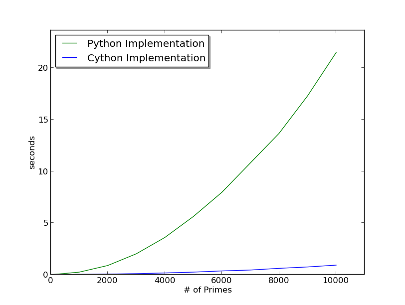
So as you can see, the partial cython implementation vastly outperforms the python function.  This gives you an idea of what kind of overhead the python interpreter brings to the language.  So know that I have a good idea of what kind of performance gains I can get using cython, I am going to try to implement some of these in my algorithms.  From what I understand, I simply need to convert python data objects to cython data types in order to get the code to compile to C.  I think a fun future project would be to write a python script that automatically converts common python data objects to their corresponding cython counterparts.  If I get a little time in the near future I may give that a shot.

So I have been playing around with Cython, which is an optimizing static compiler for Python that allows users to write python extensions in C, as a possible method to improve my algorithm performance for the discrete optimization class I have been taking.  In theory, by compiling the code before execution, the overhead associated with the python interpreter is reduced, which results in performance gains.  An additional benefit of the package is that it can run unmodified python code, so it is pretty easy to convert existing programs to cython.  I figured I would drop in my latest implementation of the Tabu Search algorithm that I wrote to solve the Traveling Salesman Problem (TSP) and compare the run-times between the two implementations.  The results of the comparison are below:

time_plot_cython

As you can (or can’t see) there is hardly a difference between the two implementations.  I was initially encouraged by the fact that the Cython implementation was running a second or two faster for the smaller TSP problems, but as the problem size increased, the time savings remained in the range of a few seconds, which doesn’t help at all.  I imagine that If I go in and re-write/translate the existing python code in the cython extension to C, I can probably see some performance gains, but merely dropping python code into a cython extension only has limited benefits.  I might go back and give this a shot, but for now I am going to keep plugging away in python.

So a few days ago I showed off some results of using a line profiler package to get detailed feedback on python programs.  Using the package, I found out that my cost calculation algorithm for a Tabu Search implementation for the Traveling Salesman Problem (TSP) was the major bottleneck in my code.  After playing around with the function and reading some forums, I figured out a way to significantly improve the cost function.  I was originally computing the cost of the entire TSP path for every 2-Opt iteration.  It turns out that this was a fairly excessive calculation, as I was only swapping the positions of two nodes at a time, the resulting change to the total cost was simply the distances between the two nodes and their respective neighbors.  So I modified the function to accept the position of the two nodes, and then calculated the distance of those partial routes to identify swaps that increased the solution’s optimality.

The original code is posted below.  In this function, I pass in a list of index values that correspond to the order in which the nodes are visited and then the function computes the total distance of the path, including the return trip to the starting point.

def calc_cost(perm):
	distance = length(points[perm[-1]], points[perm[0]])
	for i in range(0, nodeCount-1):
	    distance += length(points[perm[i]], points[perm[i+1]])
	return distance

In the modified function, shown below, I pass in the same list as before, however I added another argument to the function that indicates the position of the path that I want to evaluate. The function then calculates the distance between the provided position and the node directly before and after it in the path. I call this function four times when evaluating a 2-Opt iteration, twice to evaluate the change in the two points that were swapped, and twice again to evaluate the original distance in the path.  If the total segmented distance of the two swapped points is lower than the total segmented distance of the original two points, I keep the modified solution as it will have a lower total distance.

def calc_seg_cost(perm, c):
        if c != len(perm) - 1:
            seg = [perm[c-1], perm, perm]
        else:
            seg = [perm[c-1], perm, perm[0]]
        distance = 0
        for i in range(0, len(seg)-1):
            distance += length(points[seg[i]], points[seg[i+1]])
        return distance

I ran the two different versions of the code on a number of TSP problems and recorded the time of each run using the unix time utility.  I then plotted the results using matplotlib.

time_plot

As you can see from the plot, the function modification appears to be saving a substantial amount of time.  The primary advantage of this modification is that I can run my algorithm for a higher number of iterations and get better optimatily in the 5 hour time frame that we have.  This should help me improve my scores, but I may still need to keep tweaking the algorithm if I want to get higher scores on the larger problems, as it looks like the cost function modification by itself will not be enough to achieve that goal.

So as I mentioned in my last post, I am currently taking a discrete optimization class from Coursera.  It is a pretty challenging class, especially because I have never taken an algorithms class before (I majored in Conservation and Resource Studies in college).  I have been fairly successful in implementing some tried and true algorithms to solve some of the problem sets, but I have been having a lot of difficulty getting an understanding of the performance details of the various algorithms.  My typical routine has been to write up a few solutions to each problem, and use the run-time, solution score, and my (limited) intuition to try and improve the implementations.

In yesterday’s post I discussed a little plotting function that I wrote to help visualize my implementations to the Traveling Salesman Problem (TSP).  Today, I am going to talk about using a line profiler to get detailed feedback on the performance of your code.  I found this blog post to be very helpful in navigating the various options for performance analysis.

For the (TSP) problem, I wrote up a Tabu Search algorithm, which is a type of Local Search algorithm, that uses ‘short term memory’ to ensure that old solutions are not revisited.  While I have successfully implemented a version of the algorithm in python, I am fairly certain that I am glossing over a few key implementation details as my algorithm is not performing nearly as well as it should.  A good way to get detailed feedback on the algorithm’s performance is to use the line profiler package.  It is extremely easy to use and it provides valuable feedback on your code’s performance.  You simply add the @profile decorator to any function in your program that you want feedback on, then run a python executable at the command line (see the source blog post for details).  I threw in the profile decorator on my main Tabu function and got the following output:

Line #      Hits         Time  Per Hit   % Time  Line Contents
==============================================================
    85                                               @profile
    86                                               def search(cities, candidate_list_size, max_iter):
    87         1        13160  13160.0      0.1  	current_vector = random_permutation()
    88         1          839    839.0      0.0  	current_cost = calc_cost(current_vector)
    89         1            3      3.0      0.0  	tabu_list = []
    90         1            5      5.0      0.0  	path = [current_vector[:]]
    91     10001        30512      3.1      0.3  	for i in range(0, max_iter):
    92     10000      9332657    933.3     99.1  	    new_perm, new_cost, tabu_list = generate_candidates(current_vector, tabu_list)
    93     10000        37371      3.7      0.4  	    if new_cost < current_cost:
    94                                           		#path.append(new_perm[:])
    95        11           53      4.8      0.0  		current_vector = new_perm[:]
    96        11           34      3.1      0.0  		current_cost = new_cost
    97         1            4      4.0      0.0  	return current_vector, current_cost, path

The output of the profiler displays Hits (which is the number of times a line of code was run), Time Per Hit, and % Time. Looking at the output from the profiler, it looks like the line of code that uses the most resources is the generate_candidates function call in the main for loop (which makes sense, as the search function is basically a for loop over the generate_candidates function . So in order to take this analysis further, I added a profile decorator to the generate_candidates function and displayed the results below.

Line #      Hits         Time  Per Hit   % Time  Line Contents
==============================================================
    74                                               @profile
    75                                               def generate_candidates(best_perm, tabu_list):
    76     10000        37295      3.7      0.4  	perm = best_perm[:]
    77     10326        29927      2.9      0.3  	while True:
    78     10326       426132     41.3      4.7  	    perm = two_opt(best_perm)
    79     10326        73413      7.1      0.8  	    if perm not in tabu_list:
    80     10000        95461      9.5      1.1  		tabu_list = tabu(perm, tabu_list)
    81     10000        28268      2.8      0.3  		break
    82     10000      8269102    826.9     92.0  	perm_cost = calc_cost(perm)
    83     10000        29902      3.0      0.3  	return perm, perm_cost, tabu_list

As you can see from the output of the profiler on the generate_candidates function, the bottleneck appears to be the calc_cost function. This was not surprising as cost functions, which are used to measure the effectiveness of your solution, can be expensive to compute but are an important tool in providing your algorithm feedback in order to direct it to an optimal solution.  In this case, the cost function is a simple for loop that calculates the distance traveled in a given solution, so if I want to improve upon it, I am going to need to figure out a better way to estimate or approximate the cost without having to do the full calculation.

So know that I know where my bottleneck is, I am going to get to work on trying to find a way to improve the algorithm so that I can get some good solutions for the problem sets.  I will post an update, with some comparative metrics on performance if/when I find a way to reduce the bottleneck.