Skip navigation

Monthly Archives: July 2013

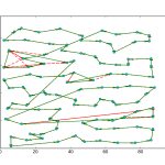
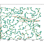
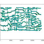
So a few days ago I showed off some results of using a line profiler package to get detailed feedback on python programs.  Using the package, I found out that my cost calculation algorithm for a Tabu Search implementation for the Traveling Salesman Problem (TSP) was the major bottleneck in my code.  After playing around with the function and reading some forums, I figured out a way to significantly improve the cost function.  I was originally computing the cost of the entire TSP path for every 2-Opt iteration.  It turns out that this was a fairly excessive calculation, as I was only swapping the positions of two nodes at a time, the resulting change to the total cost was simply the distances between the two nodes and their respective neighbors.  So I modified the function to accept the position of the two nodes, and then calculated the distance of those partial routes to identify swaps that increased the solution’s optimality.

The original code is posted below.  In this function, I pass in a list of index values that correspond to the order in which the nodes are visited and then the function computes the total distance of the path, including the return trip to the starting point.

def calc_cost(perm):
	distance = length(points[perm[-1]], points[perm[0]])
	for i in range(0, nodeCount-1):
	    distance += length(points[perm[i]], points[perm[i+1]])
	return distance

In the modified function, shown below, I pass in the same list as before, however I added another argument to the function that indicates the position of the path that I want to evaluate. The function then calculates the distance between the provided position and the node directly before and after it in the path. I call this function four times when evaluating a 2-Opt iteration, twice to evaluate the change in the two points that were swapped, and twice again to evaluate the original distance in the path.  If the total segmented distance of the two swapped points is lower than the total segmented distance of the original two points, I keep the modified solution as it will have a lower total distance.

def calc_seg_cost(perm, c):
        if c != len(perm) - 1:
            seg = [perm[c-1], perm, perm]
        else:
            seg = [perm[c-1], perm, perm[0]]
        distance = 0
        for i in range(0, len(seg)-1):
            distance += length(points[seg[i]], points[seg[i+1]])
        return distance

I ran the two different versions of the code on a number of TSP problems and recorded the time of each run using the unix time utility.  I then plotted the results using matplotlib.

time_plot

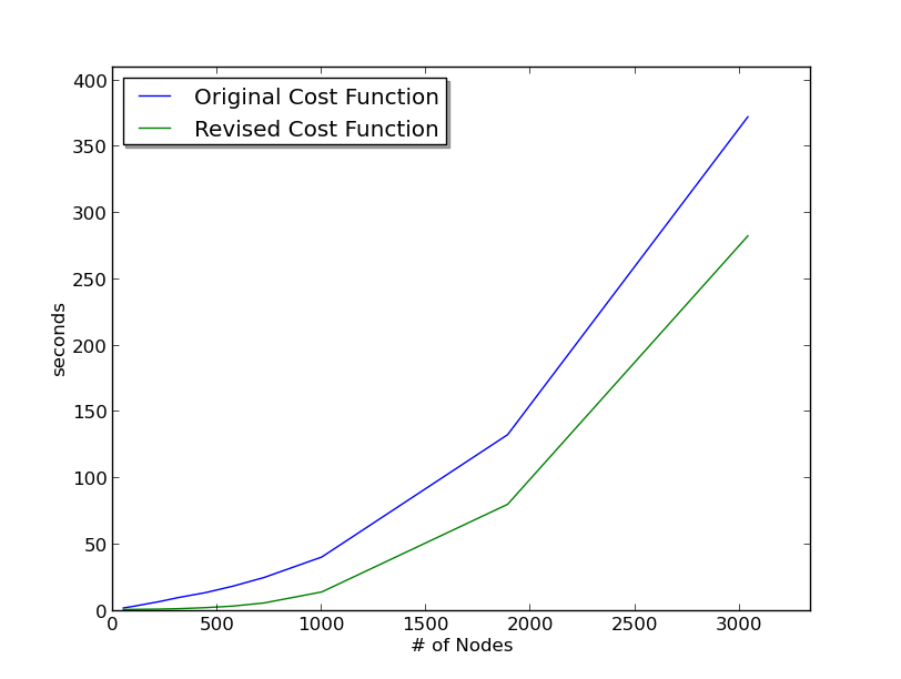
As you can see from the plot, the function modification appears to be saving a substantial amount of time.  The primary advantage of this modification is that I can run my algorithm for a higher number of iterations and get better optimatily in the 5 hour time frame that we have.  This should help me improve my scores, but I may still need to keep tweaking the algorithm if I want to get higher scores on the larger problems, as it looks like the cost function modification by itself will not be enough to achieve that goal.

So as I mentioned in my last post, I am currently taking a discrete optimization class from Coursera.  It is a pretty challenging class, especially because I have never taken an algorithms class before (I majored in Conservation and Resource Studies in college).  I have been fairly successful in implementing some tried and true algorithms to solve some of the problem sets, but I have been having a lot of difficulty getting an understanding of the performance details of the various algorithms.  My typical routine has been to write up a few solutions to each problem, and use the run-time, solution score, and my (limited) intuition to try and improve the implementations.

In yesterday’s post I discussed a little plotting function that I wrote to help visualize my implementations to the Traveling Salesman Problem (TSP).  Today, I am going to talk about using a line profiler to get detailed feedback on the performance of your code.  I found this blog post to be very helpful in navigating the various options for performance analysis.

For the (TSP) problem, I wrote up a Tabu Search algorithm, which is a type of Local Search algorithm, that uses ‘short term memory’ to ensure that old solutions are not revisited.  While I have successfully implemented a version of the algorithm in python, I am fairly certain that I am glossing over a few key implementation details as my algorithm is not performing nearly as well as it should.  A good way to get detailed feedback on the algorithm’s performance is to use the line profiler package.  It is extremely easy to use and it provides valuable feedback on your code’s performance.  You simply add the @profile decorator to any function in your program that you want feedback on, then run a python executable at the command line (see the source blog post for details).  I threw in the profile decorator on my main Tabu function and got the following output:

Line #      Hits         Time  Per Hit   % Time  Line Contents
==============================================================
    85                                               @profile
    86                                               def search(cities, candidate_list_size, max_iter):
    87         1        13160  13160.0      0.1  	current_vector = random_permutation()
    88         1          839    839.0      0.0  	current_cost = calc_cost(current_vector)
    89         1            3      3.0      0.0  	tabu_list = []
    90         1            5      5.0      0.0  	path = [current_vector[:]]
    91     10001        30512      3.1      0.3  	for i in range(0, max_iter):
    92     10000      9332657    933.3     99.1  	    new_perm, new_cost, tabu_list = generate_candidates(current_vector, tabu_list)
    93     10000        37371      3.7      0.4  	    if new_cost < current_cost:
    94                                           		#path.append(new_perm[:])
    95        11           53      4.8      0.0  		current_vector = new_perm[:]
    96        11           34      3.1      0.0  		current_cost = new_cost
    97         1            4      4.0      0.0  	return current_vector, current_cost, path

The output of the profiler displays Hits (which is the number of times a line of code was run), Time Per Hit, and % Time. Looking at the output from the profiler, it looks like the line of code that uses the most resources is the generate_candidates function call in the main for loop (which makes sense, as the search function is basically a for loop over the generate_candidates function . So in order to take this analysis further, I added a profile decorator to the generate_candidates function and displayed the results below.

Line #      Hits         Time  Per Hit   % Time  Line Contents
==============================================================
    74                                               @profile
    75                                               def generate_candidates(best_perm, tabu_list):
    76     10000        37295      3.7      0.4  	perm = best_perm[:]
    77     10326        29927      2.9      0.3  	while True:
    78     10326       426132     41.3      4.7  	    perm = two_opt(best_perm)
    79     10326        73413      7.1      0.8  	    if perm not in tabu_list:
    80     10000        95461      9.5      1.1  		tabu_list = tabu(perm, tabu_list)
    81     10000        28268      2.8      0.3  		break
    82     10000      8269102    826.9     92.0  	perm_cost = calc_cost(perm)
    83     10000        29902      3.0      0.3  	return perm, perm_cost, tabu_list

As you can see from the output of the profiler on the generate_candidates function, the bottleneck appears to be the calc_cost function. This was not surprising as cost functions, which are used to measure the effectiveness of your solution, can be expensive to compute but are an important tool in providing your algorithm feedback in order to direct it to an optimal solution.  In this case, the cost function is a simple for loop that calculates the distance traveled in a given solution, so if I want to improve upon it, I am going to need to figure out a better way to estimate or approximate the cost without having to do the full calculation.

So know that I know where my bottleneck is, I am going to get to work on trying to find a way to improve the algorithm so that I can get some good solutions for the problem sets.  I will post an update, with some comparative metrics on performance if/when I find a way to reduce the bottleneck.

So I am taking a discrete optimization class through Coursera and so far it has been pretty intense. The class uses python for it’s homework submission, so while you are free to use any language to solve the homeworks, it was easy to get up and running because python was well supported.  As I quickly found out however, the python language has a lot of overhead that slows it down considerably compared to other languages.  So I have been playing with Cython (a python package that tries to optimally compile python code to C) and have had some success with that, but will probably have to keep exploring other options as my code has been running horribly slow.

One of the recommendations from the professor was to use visualizations to help debug and improve algorithms.  I had been looking for an excuse to dive into the python plotting library matplotlib, and this seemed like a good excuse to do so. I was having trouble getting a feel for the performance of a Tabu Search implementation that I was working on for the Traveling Salesman Problems (TSP), so I decided to code something up using matplotlib to help me get a better idea of how the algorithm was working.

The TSP is a very difficult problem to optimize.  When the number of nodes gets very large, the amount of time it takes to find an optimal solution increases exponentially.  As such, it is often better to attempt to achieve sub-optimal solutions using Local Search techniques.  The downside to these algorithms, is that they rely on randomly searching for small improvements in the solution, and due to the randomness involved, it is difficult to get an idea of how your algorithm is working.  So this problem makes a fairly good candidate for developing supporting visualizations.

I took a stab at writing a simple plotting function that would plot out the nodes of the TSP problem as well as the solution path.  But I also wanted to compare the current solution with previous iterations to see how the algorithm was performing.  So I created a function that allows you to pass in as many iterations of the solutions as you like, and plots out the current solution, and overlays that on top of the older solutions in a different color.  I have used plotting libraries in R and SAS before so I figured this wouldn’t be too difficult, but as I quickly found out, and as anyone who has ever used a plotting library knows, it is pretty easy to get bogged down in documentation as each function/object has dozens of optional arguments (which is pretty standard for plotting libraries, as they need to provide the flexibility for users to create unique visualizations) and plenty of quirks.  One of the more frustrating issues that I ran into was I wanted to have arrows indicating the direction of travel to the individual nodes.  I spent a while trying to look if there was an optional line type I could use, but as I soon found out, I needed to call a special arrow object and individually draw each arrow between each point.  I was able to accomplish this with a couple of for loops, so it wasn’t a huge deal, but it definitely added to the verbosity of the code.  Anyway, the code is up on gist, here, and I have attached a few examples of the resulting output below.

There are a few things that I want to try and improve on when I get the time.  I could not find a way to lower the transparency of the arrows to represent older iterations of the solutions.  Instead, I decided to reduce the width of the red lines, however, it doesn’t seem to have a noticeable effect.  Also I wanted older iterations of the solution to have a red dashed line, but some of them appear to be solid lines.  From what I can tell, this looks like it is just an issue with the rendering.

So that’s it for today.  My next task is to play around with a line profiler to get a detailed breakdown about the performance of each line in my code.  Hopefully this will help me increase the performance of my algorithms enough to start actually getting some passing grades on the homeworks!


So I am apparently not very good at updating this blog.  I think part of the problem is I have been keeping pretty busy with Coursera classes, programming, and surfing.  When I initially started this blog, I envisioned that it would be a good way to document all of the little side projects I was working on, but I have been pretty bad about seeing these projects through to completion, so there hasn’t been much to show for the work so far.  So I am going to change directions a little bit, and probably start throwing snippets of code onto gist and write about it here.  Hopefully that will encourage me to write a few more posts!

One ‘project’ that I did manage to complete was to build a semi-functional desk from an old Ikea bed frame.  My roommate had upgraded his bed a few months ago and had initially planned on giving away or selling the old frame.  However, it just ended up sitting in a dis-assembled pile on our back porch, and I figured it would be a good idea to build something from it.  We have this weird nook in our living room that is curved, and it is difficult to efficiently use the space because most furniture items aren’t designed for that.  Additionally, due to the windows and the orientation, the space gets great natural light, so I figured it would make a good work space (I had originally setup the dining table there and was using that as a makeshift desk).

So after some back of the napkin plans my roommate and I got to work measuring, cutting, and assembling.  Out method was pretty ad hoc, and we weren’t quite sure our ‘design’ was going to actually be stable or strong enough, but after a few hours of grinding away, we ended up with something that resembled a desk!  We used the wooden slats from the bed frame to create the work surface, and offset them so that they would fit against the curve of the wall, which allowed the desk to fit snugly against the wall optimizing the space.  We cut up some of the support pieces of the bed frame for the legs.  Pictures of the before and after are below (note: the picture of the bed frame was pulled off the internet).

So after a month or two of use, I can safely say that the desk is sturdy enough (for the most part) to handle everyday use.  Some of the slats have come loose, so I need to be careful when leaning on the edge of the desk (as they might pop off).  The reason for this problem was we did not want to have screw heads exposed on the work surface, so we picked up some small screws from the hardware store and drilled through the bottom of the frame into the  bottom of the slats.  Unfortunately, our screws were a little to short, so each slat is only held on to the frame by a few screw threads, making it fairly easy to knock them loose.  I might go back with some wood glue at some point to add some extra fastening strength if the problem gets worse.

It was fun to break out the saw and the drill.  I used to build skate ramps as a young lad, and have always enjoyed woodworking, but you don’t get many opportunities for it when you live in a small-ish apartment in the middle of San Francisco.  Anyways, thanks to my roommate Will for working with this on me, hopefully I can use this desk to actually get some work done!